Basics of the Classic CNN(Convolutional Neural Network)
Basics of the Classic CNN
How a classic CNN (Convolutional Neural Network) work?
 |
Convolutional neural networks. Sounds like a weird combination of biology and math with a little CS sprinkled in, but these networks have been some of the most influential innovations in the field of computer vision and image processing.
The Convolutional neural networks are regularized versions of multilayer perceptron (MLP). They were developed based on the working of the neurons of the animal visual cortex.
Visualization of an image by a computer
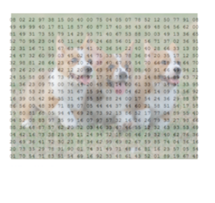
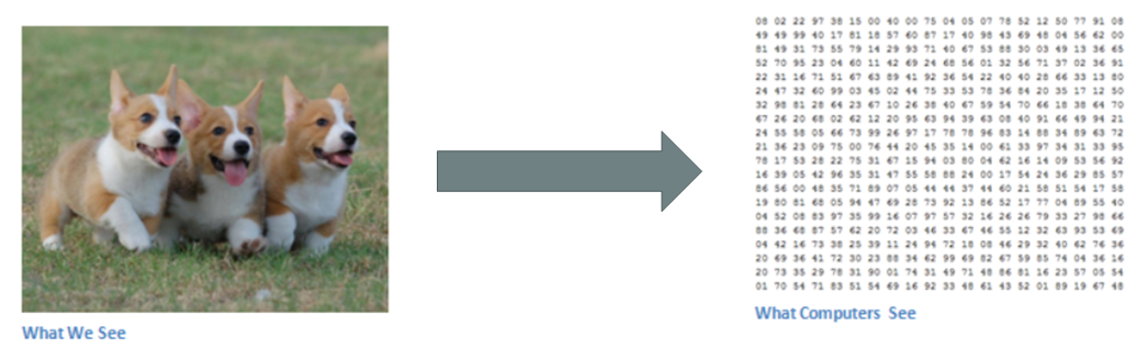 Binary image visualization.
Let’s say we have a color image in JPG form and its size is 480 x 480. The representative array will be 480 x 480 x 3. Each of these numbers is given a value from 0 to 255 which describes the pixel intensity at that point. RGB intensity values of the image are visualized by the computer for processing.
The objective of using the CNN:
The idea is that you give the computer this array of numbers and it will output numbers that describe the probability of the image being a certain class (.80 for a cat, .15 for a dog, .05 for a bird, etc.). It works similar to how our brain works. When we look at a picture of a dog, we can classify it as such if the picture has identifiable features such as paws or 4 legs. In a similar way, the computer is able to perform image classification by looking for low-level features such as edges and curves and then building up to more abstract concepts through a series of convolutional layers. The computer uses low-level features obtained at the initial levels to generate high-level features such as paws or eyes to identify the object.
A Classic CNN:
Contents of a classic Convolutional Neural Network: -
1.Convolutional Layer.
2.Activation operation following each convolutional layer.
3.Pooling layer especially Max Pooling layer and also others based on the requirement.
4.Finally Fully Connected Layer.
Convolution Operation
First Layer:
1.Input to a convolutional layer
The image is resized to an optimal size and is fed as input to the convolutional layer.
Let us consider the input as 32x32x3 array of pixel values
2. There exists a filter or neuron or kernel which lays over some of the pixels of the input image depending on the dimensions of the Kernel size.
Let the dimensions of the kernel of the filter be 5x5x3.
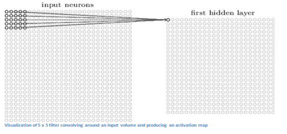
3. The Kernel actually slides over the input image, thus it is multiplying the values in the filter with the original pixel values of the image (aka computing element-wise multiplications).
The multiplications are summed up generating a single number for that particular receptive field and hence for sliding the kernel a total of 784 numbers are mapped to 28x28 array known as the feature map.
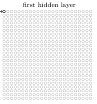
**Now if we consider two kernels of the same dimension then the obtained first layer feature map will be (28x28x2).
High-level Perspective
•Let us take a kernel of size (7x7x3) for understanding. Each of the kernels is considered to be a feature identifier, hence say that our filter will be a curve detector.
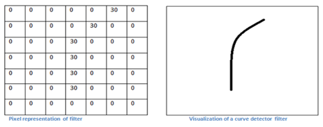
- The original image and the visualization of the kernel on the image.
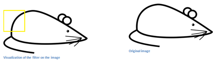
- Now when the kernel moves to the other part of the image.
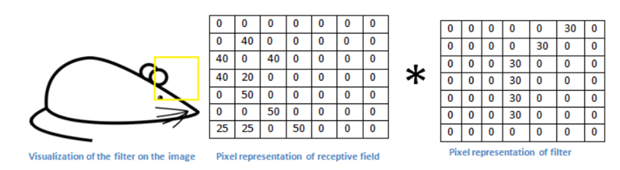
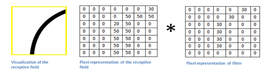
The use of the Small and the large value.
1. The value is much lower! This is because there wasn’t anything in the image section that responded to the curve detector filter. Remember, the output of this convolution layer is an activation map. So, in the simple case of a one filter convolution (and if that filter is a curve detector), the activation map will show the areas in which there at most likely to be curved in the picture.
2. In the previous example, the top-left value of our 26 x 26 x 1 activation map (26 because of the 7x7 filter instead of 5x5) will be 6600. This high value means that it is likely that there is some sort of curve in the input volume that caused the filter to activate. The top right value in our activation map will be 0 because there wasn’t anything in the input volume that caused the filter to activate. This is just for one filter.
3. This is just a filter that is going to detect lines that curve outward and to the right. We can have other filters for lines that curve to the left or for straight edges. The more filters, the greater the depth of the activation map, and the more information we have about the input volume.
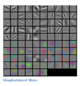
In the picture, we can see some examples of actual visualizations of the filters of the first conv. layer of a trained network. Nonetheless, the main argument remains the same. The filters on the first layer convolve around the input image and “activate” (or compute high values) when the specific feature it is looking for is in the input volume.
Sequential conv. layers after the first one.
1.When we go through another conv. layer, the output of the first conv. layer becomes the input of the 2nd conv. layer.
2. However, when we’re talking about the 2nd conv. layer, the input is the activation map(s) that result from the first layer. So each layer of the input is basically describing the locations in the original image for where certain low-level features appear.
3. Now when you apply a set of filters on top of that (pass it through the 2nd conv. layer), the output will be activations that represent higher-level features. Types of these features could be semicircles (a combination of a curve and straight edge) or squares (a combination of several straight edges). As you go through the network and go through more conv. layers, you get activation maps that represent more and more complex features.
4. By the end of the network, you may have some filters that activate when there is handwriting in the image, filters that activate when they see pink objects, etc.
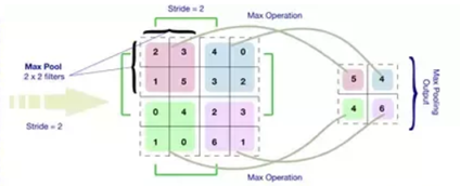
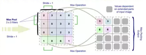
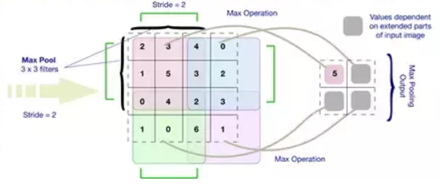
Pooling Operation.
Max Pooling example.
Fully Connected layer.
1.The way this fully connected layer works is that it looks at the output of the previous layer (which as we remember should represent the activation maps of high-level features) and the number of classes N (10 for digit classification).
2. For example, if the program is predicting that some image is a dog, it will have high values in the activation maps that represent high-level features like a paw or 4 legs, etc. Basically, an FC layer looks at what high level features most strongly correlate to a particular class and has particular weights so that when you compute the products between the weights and the previous layer, you get the correct probabilities for the different classes.
3. The output of a fully connected layer is as follows [0 .1 .1 .75 0 0 0 0 0 .05], then this represents a 10% probability that the image is a 1, a 10% probability that the image is a 2, a 75% probability that the image is a 3, and a 5% probability that the image is a 9 (Softmax approach) for digit classification.
Training.
§We know kernels also known as feature identifiers, used for identification of specific features. But how the kernels are initialized with the specific weights or how do the filters know what values to have.
Hence comes the important step of training. The training process is also known as backpropagation, which is further separated into 4 distinct sections or processes.
•Forward Pass
•Loss Function
•Backward Pass
•Weight Update
The Forward Pass:
For the first epoch or iteration of the training the initial kernels of the first conv. layer is initialized with random values. Thus after the first iteration output will be something like [.1.1.1.1.1.1.1.1.1.1], which does not give preference to any class as the kernels don’t have specific weights.
The Loss Function:
The training involves images along with labels, hence the label for the digit 3 will be [0 0 0 1 0 0 0 0 0 0], whereas the output after a first epoch is very different, hence we will calculate loss (MSE — Mean Squared Error)
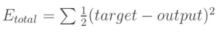
The objective is to minimize the loss, which is an optimization problem in calculus. It involves trying to adjust the weights to reduce the loss.
The Backward Pass:
It involves determining which weights contributed most to the loss and finding ways to adjust them so that the loss decreases. It is computed using dL/dW, where L is the loss and the W is the weights of the corresponding kernel.
The weight update:
This is where the weights of the kernel are updated using the following equation.
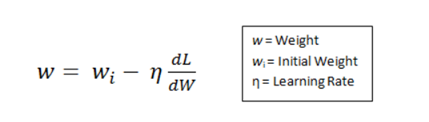
Here the Learning Rate is chosen by the programmer. Larger value of the learning rate indicates much larger steps towards optimization of steps and larger time to convolve to an optimized weight.
Testing.
Finally, to see whether or not our CNN works, we have a different set of images and labels (can’t double dip between training and test!) and pass the images through the CNN. We compare the outputs to the ground truth and see if our network works!


Comments
Post a Comment